Carnegie Mellon University Robotics Institute logo
CMU Robotics Institute · SURG Research Project

Badminton Shuttle Collection System

An autonomous ground robot that finds every shuttlecock scattered across a badminton court, works out the shortest route to reach them, and collects them — so players don't have to. This project combines instance-segmentation detection, camera-to-world coordinate transforms, and a greedy TSP traversal strategy that outperforms standard path-planning baselines on this task.

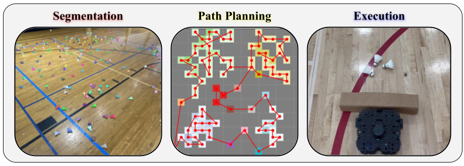
Three-panel summary: segmentation masks over shuttlecocks on a court, a discretized-grid TSP path plan, and the robot executing collection on court

Why this exists

After a badminton training session, dozens of shuttlecocks end up scattered across the court and have to be picked up by hand. This project builds a mobile robot that automates that job: an onboard camera detects shuttles, a coordinate transform maps each detection onto real-world court coordinates, and a path planner sequences them into a route the robot can actually drive — before a particle-filter localization and pure-pursuit control stack executes it.

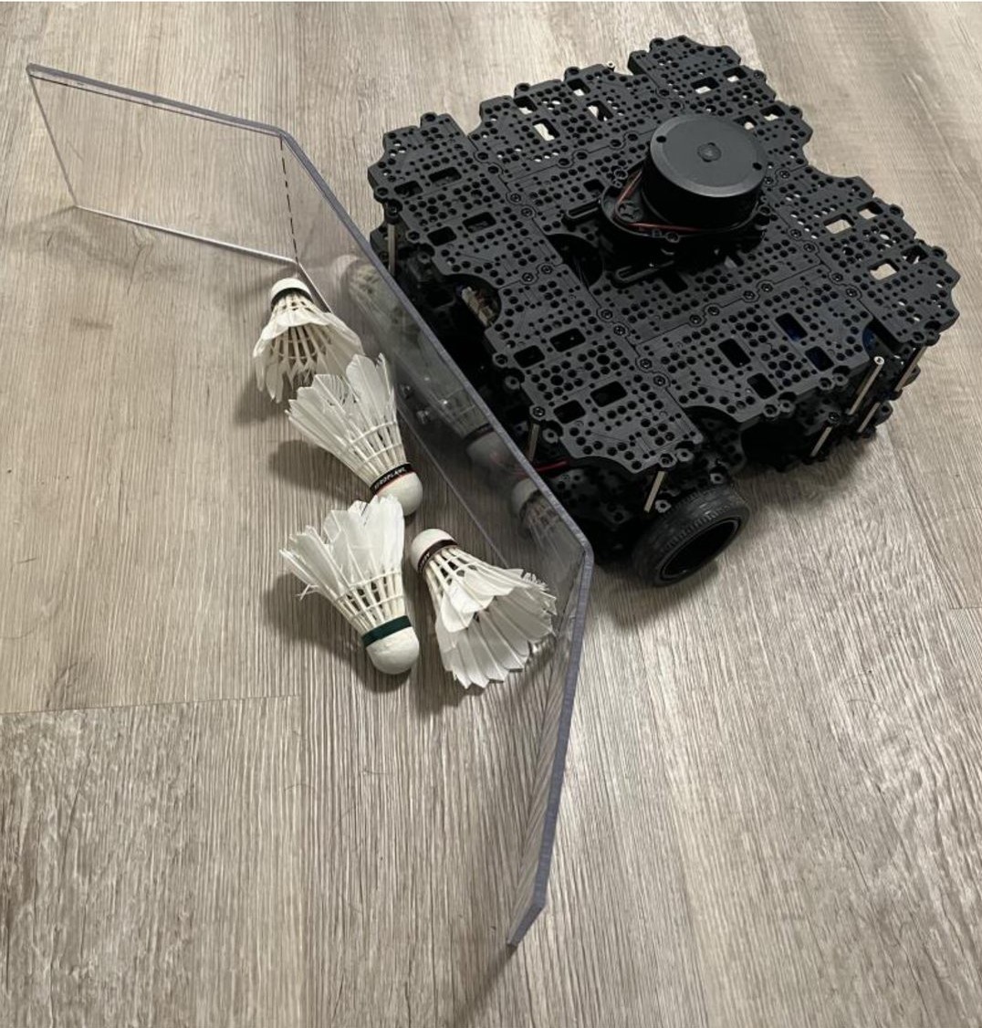
The collection robot next to three badminton shuttlecocks on a wood floor
The robot. A differential-drive collection robot, 3D-printed and assembled with help from the CMU RI Workshop.
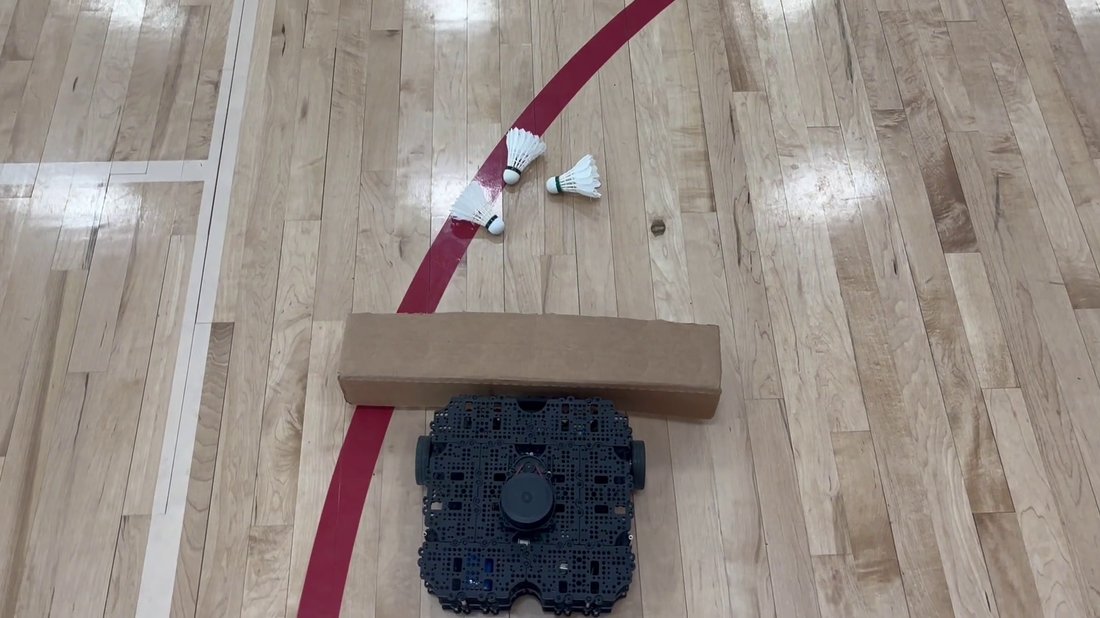
Overhead view of the robot with a cardboard collection ramp approaching shuttlecocks on court
On court. A frame from the real-world demo run below — the robot closing in on a pair of shuttles.
Detectron2 / Mask R-CNN Camera calibration & perspective transform Grid discretization & clustering Greedy TSP routing Particle filter localization Pure pursuit control Gazebo simulation

End-to-end pipeline

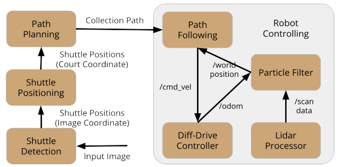
Shuttle detections flow from image coordinates to court coordinates to a collection path, which a particle filter and differential-drive controller then execute in closed loop with LiDAR and odometry feedback.

Block diagram: Shuttle Detection feeds Shuttle Positioning feeds Path Planning feeds Path Following, which exchanges cmd_vel and odom with a Diff-Drive Controller and world position with a Particle Filter fed by a Lidar Processor

Detection & coordinate transform

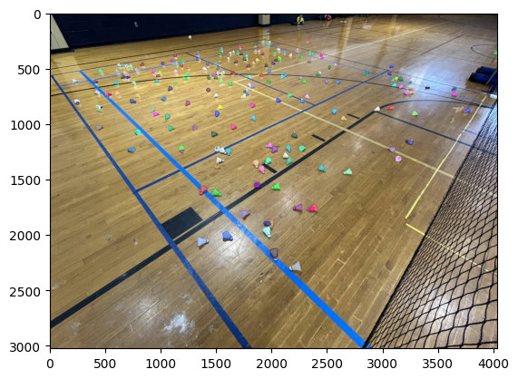
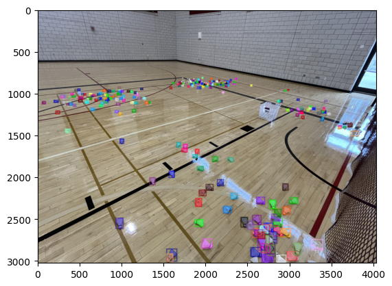
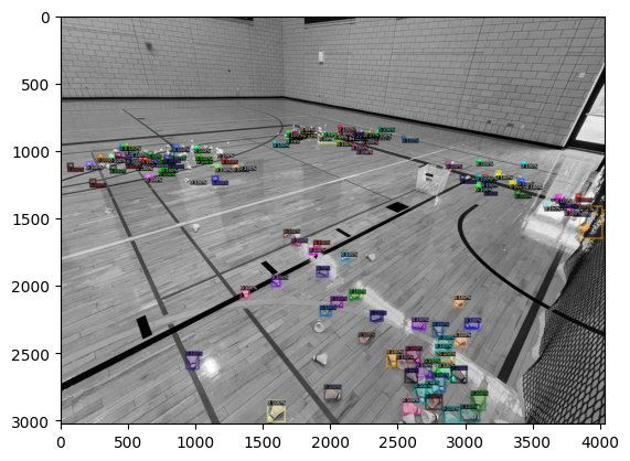
prediction.py runs sliding-window instance segmentation with a customized Mask R-CNN model (Detectron2, trained in training.py on data labeled with Label Studio) to locate shuttlecocks in a raw frame. coordinate_transform.py then uses a calibrated camera matrix plus an optimized roll/yaw/displacement transform to project each detection from image pixels onto a flat, real-world court coordinate system.

Mask R-CNN sliding-window detection overlaid on a photo of scattered shuttlecocks on a badminton court
Sliding-window detection. Each colored mask is one detected shuttlecock, sampled on a real court.
Segmentation masks over dozens of scattered shuttlecocks on a gym floor
Dense scatter. The model holds up under heavy clutter and specular floor reflections.
Bounding boxes with class labels and confidence scores over shuttlecocks scattered across a gymnasium
Bounding boxes & scores. Per-instance class and confidence output across a full-court view.
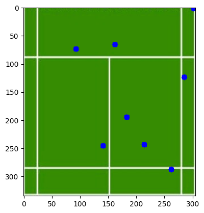
Detected shuttlecock positions plotted on a flat court diagram after coordinate transform
Coordinate transform. The same detections re-projected onto real-world court coordinates, ready for path planning.

Shuttle positioning

$$\vec{s} = K^{-1}\theta_{img}$$ $$\theta_{cam} = z\vec{s}$$ $$\theta_{world} = R^{T}\theta_{cam} + C$$ $$z = -\dfrac{C_z}{R_{*2}^{T}\vec{s}}$$
  • A shuttle's image-space position $\theta_{img}$ is unprojected into a ray of possible camera-space positions, then transformed into court coordinates $\theta_{world}$ using the camera's pose $(R, C)$.

Particle filter (localization)

$$\theta_{MLE} = \operatorname*{arg\,max}_{t} P(t \mid D)$$ $$t = t + m + n$$
  • $D$ = LiDAR scan, $t$ = particle position
  • $m$ = motion, $n \sim \mathcal{N}(\vec{0}, \sigma)$ = motion noise
  • Odometry proposes motion; LiDAR returns off the court poles correct drift.

Pure pursuit (path following)

$$\gamma = \dfrac{2 \times \sin(\Delta\alpha)}{d}$$ $$\omega = \gamma v$$
  • $\Delta\alpha$ = angular difference, $d$ = lookahead distance
  • $\gamma$ = curvature, $v$ = linear velocity, $\omega$ = angular velocity

Path planning: greedy TSP over discretized clusters

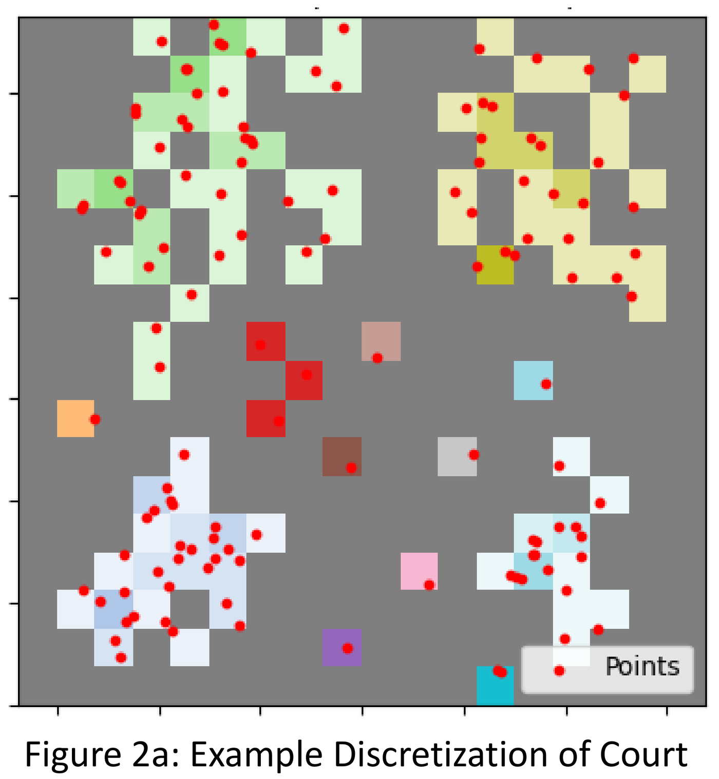
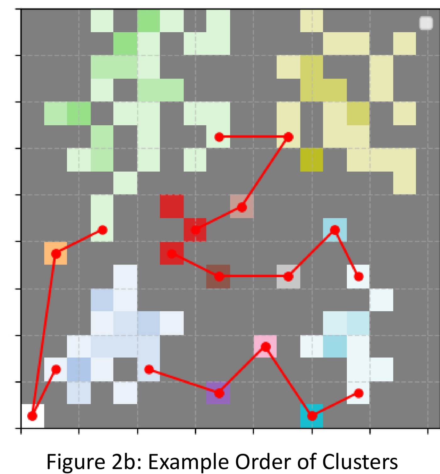
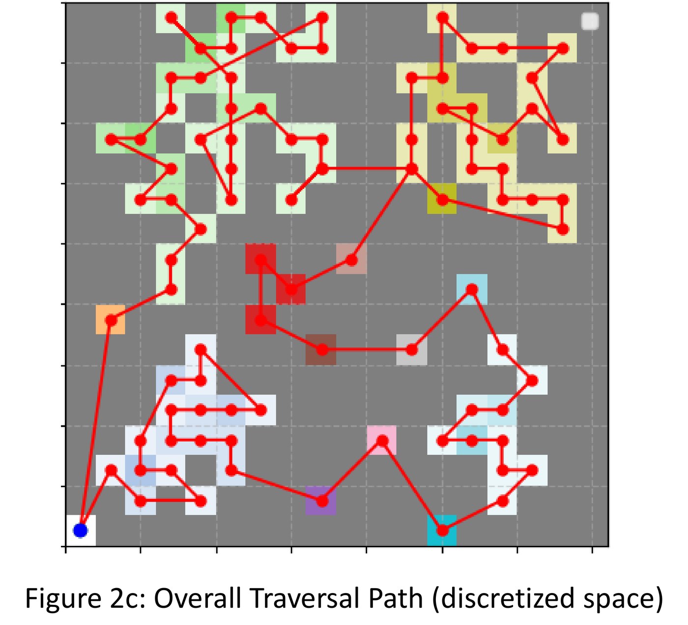
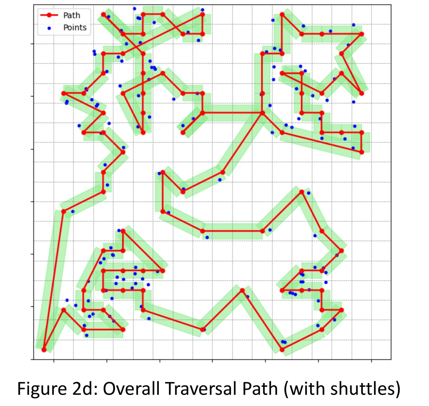
Once the robot sweeps through a region of the court, every shuttle inside it is collected — so the court is discretized into square cells the width of the collector, and connected cells are grouped into clusters. A fully-connected graph of clusters is built from inter-cluster distances, and the visiting order is chosen by solving a Travelling Salesman Problem over that graph. Within each cluster, a second TSP orders the individual shuttles, and the results are stitched into one overall path.

Court discretized into colored square cells, each grouping nearby detected shuttles
1. Discretize. The court is binned into cells the width of the collector; connected cells form clusters.
Red path connecting the centers of each cluster in visiting order
2. Order clusters. TSP over the cluster graph picks a short visiting order between clusters.
Full traversal path threading through every cluster in discretized grid space
3. Order within clusters. A second TSP sequences shuttles inside each cluster; the results connect into one path.
Overall traversal path overlaid on the original scattered shuttle positions, with the collector's swept width highlighted
4. Final path. The stitched route, with the collector's swept width shown, covering every shuttle on the court.

Localization & control

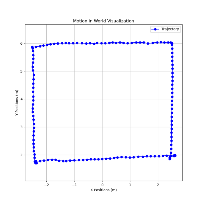
A particle filter fuses wheel odometry with LiDAR returns off the court's boundary poles to keep the robot localized, while a pure-pursuit controller follows the planned path by steering toward a lookahead point along it. Both were validated in a Gazebo simulation of the court before running on hardware.

LiDAR-assisted localization trajectory plotted over the court
LiDAR-assisted localization. Estimated robot trajectory while tracing the court boundary.
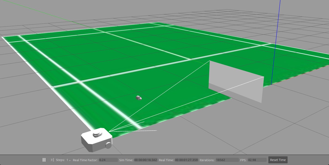
Gazebo simulation of the collection robot on a modeled badminton court
Gazebo simulation. The robot and court modeled in simulation for path-following tests before hardware runs.

Watch it run

The full stack — detection, coordinate transform, path planning, localization, and control — running on hardware on a real court.

Real-world demo. The robot approaching shuttles on court, guided by a cardboard collection ramp.

Greedy TSP vs. standard baselines

Shuttle patterns were randomly scattered on the court and photographed; the same pattern was replayed for each path-planning algorithm so results are directly comparable. Distance travelled and time spent were logged by the robot, and accuracy is the percentage of shuttles actually collected by the end of the run.

Path modelDistance travelled (m)Time spent (s)Accuracy
Greedy TSP8.8949100%
Standard TSP9.034892.3%
Nearest Neighbor9.5055100%
Ox Turn25.03134100%

The greedy TSP algorithm matches standard TSP's distance and time while avoiding its shuttle losses from frequent large-angle turns, and it clearly outperforms simpler Nearest Neighbor and Ox Turn (sweep coverage) baselines on this collection task.

Repository structure

The pipeline can be run end-to-end via pipeline.py, which chains detection, coordinate transform, and traversal planning on a test image.

prediction.py              Mask R-CNN sliding-window detection (Detectron2)
training.py                Trains the shuttle-detection model
coordinate_transform.py    Camera calibration + image-to-court coordinate transform
pipeline.py                End-to-end: detect → transform → plan
traveral_algorithm.py      Combines traversal strategies into one pipeline
path_planning.py           Grid discretization & connected-component clustering
k-mean_clustering.py       K-means clustering of shuttle positions
minimum_cost_flow.py       Weighted balanced clustering via min-cost flow
integer_linear_programming.py  ILP / TSP route optimization
spine_tree_cluster_traversal.py  Tree-based cluster traversal heuristic
state_space.py             Robot pose belief & target-visibility model
Images/, Labels/, datasets/  Training data, annotations, and captured test imagery
logs/                      Training run configs, metrics, and checkpoints